
Another underused feature of Excel is Named Ranges. Named Ranges allow you to assign a meaningful name to a cell or a range of cells and then use that name instead of the actual cell reference in your formulas. A name is easier to remember when you are constructing your formulas.
Creating a named range
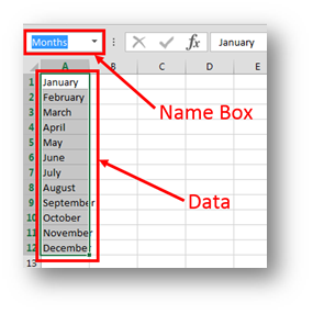
Select one or more cells, and then click in the Name Box. It’s located left of the formula bar at the top of the worksheet, below the Ribbon. If you’re not sure you’re in the right place, hover and the Name Box tip will pop up.
Top 3 Reasons to Use Named Ranges in Excel
i) Data Validation
Using a named range to create a dropdown list in a cell makes data entry easier and cleaner.
Without a named range, the list of acceptable choices must be in the same worksheet as the target cell. Using a named range allows you to put that list anywhere in your workbook.
Making a tab called “lists,” which holds all the named ranges used in selection lists, is helpful.
- From the Data tab, in the Data Tools group, choose the Data Validation button.
- Choose List selection in the Allow: field.
- In the Source field type an “=” and the name of your range as illustrated.
The easiest mistake to make here is to forget the equals sign.

ii) Formulas
A named range is the best choice when using an Absolute Cell Reference ($A$1) to refer your formula to the exact same cell (no matter where it’s copied).
In a VLookUp, for example, forgetting to set your Table Array to an absolute cell reference range can yield unpredictable results.

Simply setting a name range for your table array makes worrying about an absolute cell reference unnecessary. Even naming single cells can be helpful in creating a self-documenting formula.
For example, assume you have a workbook that contains a lot of formulas that contain a tax rate. You could simplify things by using one cell to store the tax rate, naming that cell ‘CommissionRate‘ and then, instead of using the cell reference in your formulas, you would use the name ‘CommissionRate‘.
Try this:
- Enter 12% (Commission Rate) in cell C2.
- To name the cell, select Insert, Name, Define.
- Type ‘CommissionRate‘ and click OK.
- Now, in cells C5:C8 enter some numbers.
- In cell D5 enter the formula =+C5*CommissionRate and copy it down to cells D6:D8.
Using Named ranges help you to create easier to understand and well organized workbooks. Now whenever you need to change the Commission Rate, you just change it in one cell and all dependent formulas are instantly updated.
iii) Bookmarks
If you have elaborate workbooks, which contain target figures like net profit, average cost and gross income, you can highlight the result cells and name them for what they represent. Then, click in the name box from anywhere in the workbook, select the name, and it will take you there.
Also Read: